PeakPacer: Optimizing Cycling Performance
One of the most important factors that cycling time trial athletes need to consider is how to pace themselves during the race. The challenge can be summarized as follows: the cyclist has limited energy that must be partitioned efficiently to maximize the average velocity over a given race course. In this article, we will first discuss the theoretical physics of cycling and, leveraging that knowledge, present an application capable of computing the optimal power profile for minimizing travel time on a course. The application uses a GPS track and the rider's and weather characteristics. We will also explore how to experimentally determine the rider's CdA (Coefficient of Drag Area) for simplifying field testing.
Theory
Building a model to predict the optimal power curve that minimizes travel time on a GPS track is a complex problem. It can be broken down into two main parts:
- Establish a power-speed relationship (and vice versa).
- Maximize the average speed along the course based on parameters dependent on the course, given a power profile for the athlete.
Here, we will demonstrate the simplest possible model, but more complex models are available in the literature.
Power-Velocity Relationship
We will use a simplified model that estimates the power required by a cyclist as the sum of the resistances encountered during the ride. A more detailed model can be derived from Martin, James C., et al.'s study titled "Validation of a mathematical model for road cycling power" (Journal of Applied Biomechanics, 1998). However, for simplicity, we will focus on the four main resistances:
- Aerodynamic force
- Rolling resistance
- Gravity
- Overall bike efficiency
Aerodynamic Force
Aerodynamic force is the resistance cyclists face as they move through the air. It can be estimated using the following parameters:
- v: Cyclist's speed
- ρ: Air density (ρ = 1.292 kg/m³)
- CdA: Aerodynamic drag coefficient (e.g., TT: 0.25; aerodynamic road position: 0.30; relaxed road position: 0.33)
- vwind: Wind speed (positive for headwind)
The formula for the aerodynamic force is:
\[ F_a = \frac{1}{2} \rho \cdot \text{CdA} \cdot (v + v_{\text{wind}})^2 \]
Rolling Resistance
Rolling resistance is the cyclist's resistance due to the contact between the tires and the road. It can be estimated using the following parameters:
- Crr: Coefficient of rolling friction (e.g., wood track: 0.0020; good asphalt: 0.0040; worn asphalt: 0.0045)
- m: Total weight (cyclist + bike + equipment)
- α: Road slope expressed as a percentage
- g: Gravitational acceleration (9.8067 m/s²)
The formula for rolling resistance is:
\[ F_r = \text{Crr} \cdot m \cdot g \cdot \cos \left( \arctan(0.01 \cdot \alpha) \right) \]
Gravitational Force
Gravitational force is the force a cyclist must overcome when riding uphill. It can be estimated using the following parameters:
- v: Cyclist's speed
- m: Total weight (cyclist + bike + equipment)
- α: Road slope expressed as a percentage
- g: Gravitational acceleration (9.8067 m/s²)
The formula for gravitational force is:
\[ F_g = m \cdot g \cdot \sin \left( \arctan(0.01 \cdot \alpha) \right) \]
Propulsion Power
The propulsion power is the force required to counteract the effects of air resistance, road friction, and gravity. To account for energy loss through transmission and bearings, we increase the required power by a coefficient of 2-3%. This can be referenced in the work by Jeukendrup, Asker E, and James Martin in their 2001 paper "Improving Cycling Performance" (Sports Medicine 31 (7): 559–69).
The propulsion power can be estimated using the following parameters:
- v: Cyclist's speed
- ρ: Air density (~1.292 kg/m³)
- CdA: Aerodynamic drag coefficient (e.g., CLM: 0.25; aerodynamic road position: 0.30; relaxed road position: 0.33)
- vwind: Wind speed (positive for headwind)
- Crr: Rolling friction (wood track: 0.0020; good asphalt: 0.0040; worn asphalt: 0.0045)
- m: Total weight (cyclist + bike + equipment)
- α: Road slope expressed as a percentage
- Eff: Efficiency (0.97 to 0.98)
The formula for propulsion power is:
\[ P_P = v \cdot \text{Eff} \cdot \left( F_a + F_r + F_g \right) \]
\[ P_P = v \cdot \text{Eff} \cdot \left[ \frac{1}{2} \cdot \rho \cdot \text{CdA} \cdot (v + v_{\text{wind}})^2 + \text{Crr} \cdot m \cdot g \cdot \cos\left( \arctan(0.01 \cdot \alpha) \right) + m \cdot g \cdot \sin\left( \arctan(0.01 \cdot \alpha) \right) \right] \]
The formula for the velocity given a propulsion power is:
\[ \frac{1}{2} \cdot \rho \cdot \text{CdA} \cdot \text{Eff} \cdot v^3 + \rho \cdot \text{CdA} \cdot \text{Eff} \cdot v_{\text{wind}} \cdot v^2 + \left( \frac{1}{2} \cdot \rho \cdot \text{CdA} \cdot \text{Eff} \cdot v_{\text{wind}}^2 + \text{Eff} \cdot \left[ \text{Crr} \cdot m \cdot g \cdot \cos\left( \arctan(0.01 \cdot \alpha) \right) + m \cdot g \cdot \sin\left( \arctan(0.01 \cdot \alpha) \right) \right] \right) \cdot v - P_P = 0 \]
Optimal Power Profile
Finding the optimal power profile involves minimizing travel time (maximizing average speed) by maximizing available athlete energy. The optimal solution where wind and slope vary along the course can be difficult to obtain. A simplified solution can be derived without wind, using Pontryagin's principle (De Jong, Jenny, et al., "The individual time trial as an optimal control problem", 2017).
In the following, we will use a method that can consider all the factors. This method will discretize the course into segments (e.g., every 10 meters or at every change in direction or road gradient) and optimize travel time on these segments using Sequential Quadratic Programming (SLSQP) to minimize the total travel time. The optimization process requires solving cubic equations to find the velocity given a power.
It's evident that at each minimization step, the algorithm will need to solve a cubic equation for each segment, which is computationally intensive. Fortunately, we can apply Cardano's formula to solve cubic equations, significantly reducing the time complexity of the solution.
\[ v = \sqrt[3]{ -\frac{1}{2} \cdot q + \sqrt{ \left( \frac{q}{2} \right)^2 + \left( \frac{p}{3} \right)^3 } } + \sqrt[3]{ -\frac{1}{2} \cdot q - \sqrt{ \left( \frac{q}{2} \right)^2 + \left( \frac{p}{3} \right)^3 } } - \frac{ \rho \cdot \text{CdA} \cdot \text{Eff} \cdot v_{\text{wind}} }{ 3 \cdot \left( \frac{1}{2} \cdot \rho \cdot \text{CdA} \cdot \text{Eff} \right) } \] \[ \text{where:} \] \[ p = \frac{ 3 \cdot \left( \frac{1}{2} \cdot \rho \cdot \text{CdA} \cdot \text{Eff} \right) \cdot \left( \left( \frac{1}{2} \cdot \rho \cdot \text{CdA} \cdot v_{\text{wind}}^2 + B \right) \cdot \text{Eff} \right) - \left( \rho \cdot \text{CdA} \cdot \text{Eff} \cdot v_{\text{wind}} \right)^2 }{ 3 \cdot \left( \frac{1}{2} \cdot \rho \cdot \text{CdA} \cdot \text{Eff} \right)^2 } \] \[ q = \frac{ 2 \cdot \left( \rho \cdot \text{CdA} \cdot \text{Eff} \cdot v_{\text{wind}} \right)^3 - 9 \cdot \left( \frac{1}{2} \cdot \rho \cdot \text{CdA} \cdot \text{Eff} \right) \cdot \left( \rho \cdot \text{CdA} \cdot \text{Eff} \cdot v_{\text{wind}} \right) \cdot \left( \left( \frac{1}{2} \cdot \rho \cdot \text{CdA} \cdot v_{\text{wind}}^2 + B \right) \cdot \text{Eff} \right) + 27 \cdot \left( \frac{1}{2} \cdot \rho \cdot \text{CdA} \cdot \text{Eff} \right)^2 \cdot (-P_P) }{ 27 \cdot \left( \frac{1}{2} \cdot \rho \cdot \text{CdA} \cdot \text{Eff} \right)^3 } \] \[ B = \text{Crr} \cdot m \cdot g \cdot \cos\left( \arctan(0.01 \cdot \alpha) \right) + m \cdot g \cdot \sin\left( \arctan(0.01 \cdot \alpha) \right) \]
Additionally, we can impose power constraints based on the athlete's power profile—such as limiting sustained efforts to avoid exceeding their Maximum Aerobic Power (MAP) over a 5-minute interval—and introduce smoothness constraints on both power and velocity profiles. These constraints and optimizations can efficiently solve the minimization problem, even on long or complex race courses.
\[ \begin{aligned} & \min_{P_i} && \sum_{i=1}^{N} \frac{\Delta x_i}{v_i(P_i)} \quad \text{(minimize total time)} \\ \\ & \text{subject to:} \\ & && \frac{\sum_{i=1}^{N} P_i \cdot \frac{\Delta x_i}{v_i(P_i)}}{\sum_{i=1}^{N} \frac{\Delta x_i}{v_i(P_i)}} \leq P_{\text{target}} \quad \text{(mean power constraint)} \\ \\ & && \max_{t \in [0, T-300]} \left( \frac{1}{300} \sum_{j=t}^{t+299} P_j \right) \leq 0.95 \cdot \text{PMA} \quad \text{(5-min power constraint)} \\ \\ & && 0.25 \cdot \text{PMA} \leq P_i \leq 1.5 \cdot \text{PMA} \quad \text{for all } i = 1, \dots, N \quad \text{(power bounds)} \end{aligned} \]
I employ a simplified constraint model where the target power along the course is derived from the athlete's Functional Threshold Power (FTP) using the well-established hyperbolic power-duration relationship. The parameters of this function can be approximated from the athlete's FTP; however, a more accurate approach would involve using the concept of Critical Power (CP). For more details, see my article on the 3-minute all-out test, which describes how CP can determine the maximum sustainable power over varying durations.
For longer efforts, it is often more appropriate to use normalized power as a constraint instead of mean power. Normalized power (NP) accounts for the variability in effort and provides a more physiologically representative estimate of the actual energy cost of an effort. It is calculated by applying a weighted rolling average of the 30-second power over the entire ride and then taking the fourth root of the average of those values raised to the fourth power. This value sometimes better reflects the physiological stress experienced by the rider.
The model also incorporates the athlete's MAP to ensure that the rolling average power over any 5-minute window does not exceed 95% of this value. By applying these two hard constraints (based on FTP and MAP), I have experimentally observed that the optimized pacing strategy resembles how experienced riders tend to adopt intuitively. A more rigorous approach using the CP and a constraint matching the entire power-duration profile of an athlete should be possible. Still, in practice, the simpler model is largely sufficient, allowing room to adapt to the day's form and other uncertain circumstances.
CdA (Coefficient of Drag Area)
Using the formula above, if we know the power, weather conditions, and velocity, we can compute the rider's and bike's CdA for a given wind orientation. This can be used to display the CdA versus the yaw angle of the cyclist and be used to optimize rider position and material choice using field tests.
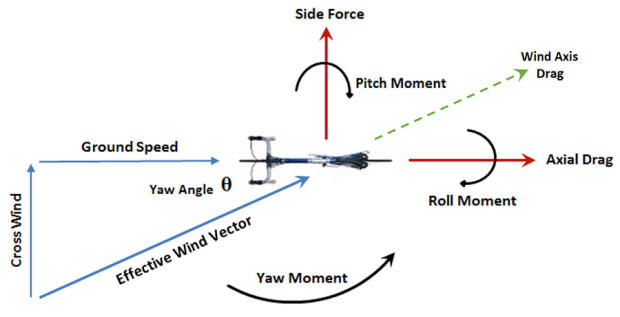
Yaw angle in cycling refers to the angle between the direction of the wind and the direction the cyclist is traveling. It is a crucial factor in aerodynamics:
- A yaw angle of 0° means the wind is directly head-on.
- As the wind shifts more to the side, the yaw angle increases (typically up to 15–20° in real-world conditions).
- A higher yaw angle affects how air flows around the cyclist and the bike, influencing aerodynamic drag.
PeakPacer
Leveraging the theory discussed above, I have developed a tool called PeakPacer that can:
- Compute the optimal power profile to minimize travel time on a given course.
- Compute the CdA of a rider and bike from a FIT file containing power and velocity data.
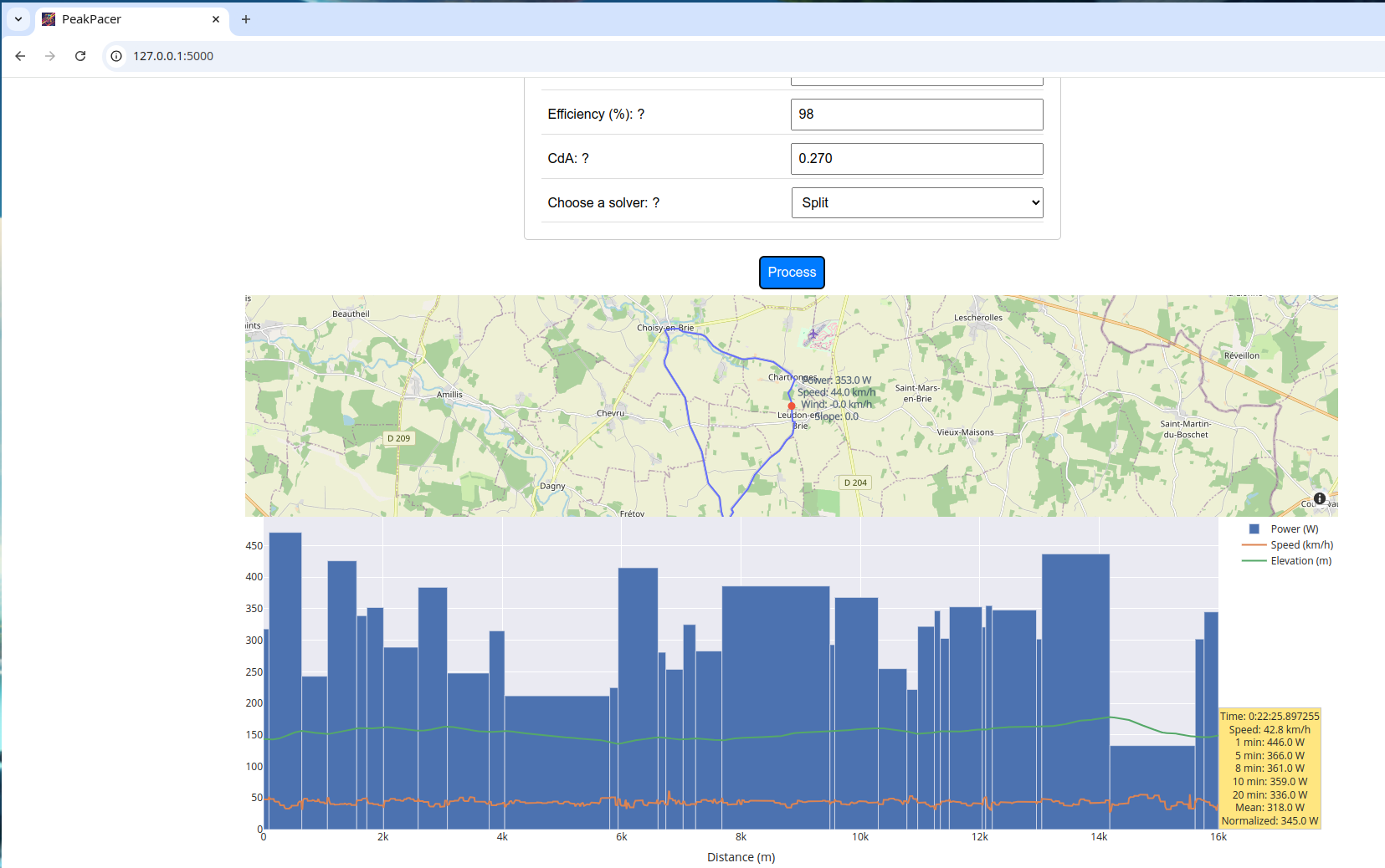
Optimal Power Profile with PeakPacer
PeakPacer can output the optimal power profile based on the course and rider's profile. The rider's profile should include:
- Total rider and bike weight
- Rider FTP (Functional Threshold Power, the power the rider can maintain for 1 hour)
- Rider MAP (Maximum Aerobic Power, the power the rider can sustain for 5 minutes)
- Rider/bike efficiency
- Rider/bike CdA
The tool also requires the road profile, which can be provided as a GPX file. The optimization algorithm will consider segments of the course based on direction changes, gradient changes, or constant segment size depending on the chosen solver. The wind speed, direction, temperature, pressure, humidity, and rolling friction coefficient must also be provided.
With these parameters, PeakPacer will optimize the power profile to minimize travel time, maximizing the energy available according to the rider's power profile.
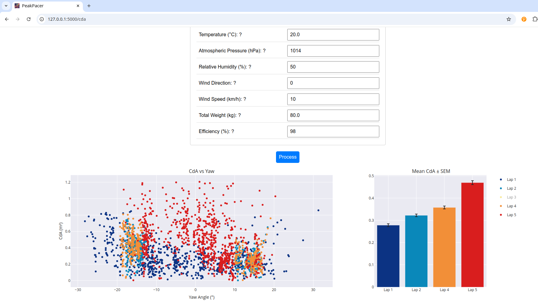
CdA Estimation with PeakPacer
PeakPacer can simplify field testing by providing an estimation of CdA based on a given yaw angle. To perform the CdA estimation, the tool needs a FIT file with GPS trace, velocity, rider power, and road, rider, and weather data, as described earlier. The tool computes the CdA at various points along the course and averages the results to estimate the CdA based on the yaw angle.
Conclusion
We have explored the basic theory of cycling modeling using simple physics. By combining this theory with a minimization technique, we have created a tool to predict the optimal power profile needed to minimize travel time on a given course. PeakPacer offers cyclists an invaluable resource for optimizing their performance during time trials.